

| Foreword: Styles Toolbox, Moving Forward in 2023, Continues to be Updated with 4 New Advanced ArcGIS Mapping Styles! |
GIS Mapping Toolbox, updated February 2023 with 4 new mapping effects. By the current version, 18 tools have been included.
1.New tools
Four new mapping style tools have been added: Plane Diagonal Chart, Light and Dark Contours, Three Dimensional Elements, and Background Blur.
1.1Plane oblique axes diagram
Plan oblique is a method of graphic projection in which objects are projected onto a plane oblique to the observer.
Plan oblique projection is commonly used in architectural and engineering drawings to show the depth and spatial relationships of objects.
But here we apply it to DEM data.
The default tilt angle is 35 degrees, and you can fill in different tilt angles to control the stereoscopic height of the resulting oblique map in the Y-axis.
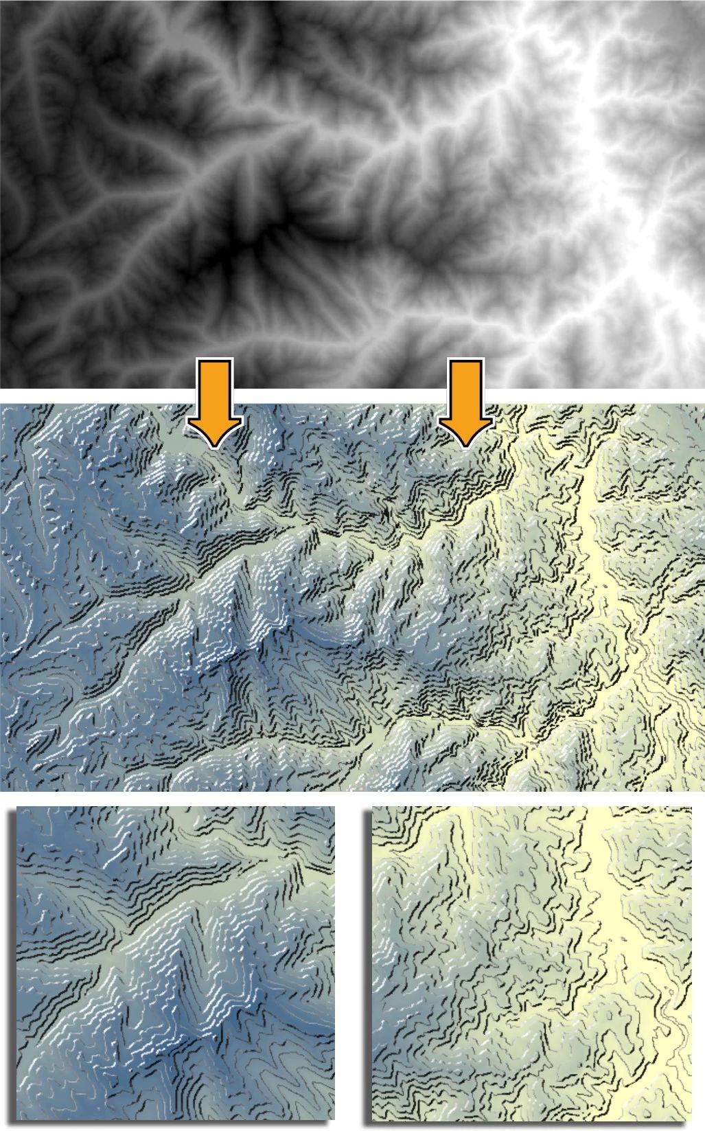
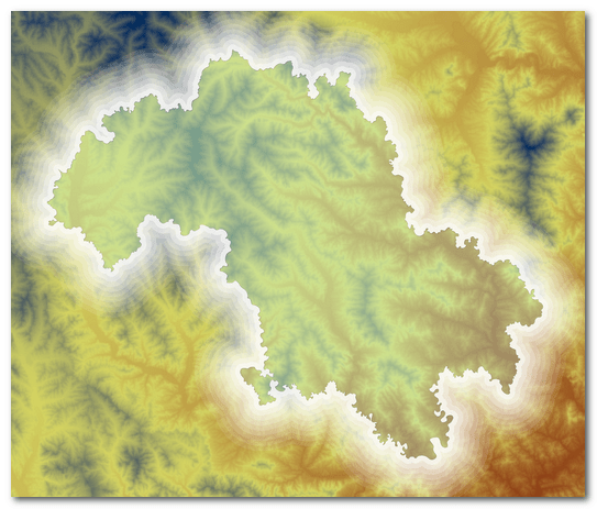
1.2light and dark contours
Use light and dark contour lines ( illuminated contour)The method of geomorphological expression was first invented by the Japanese cartographer Kitiro Tanaka and has been unanimously recognized by the cartographic community, so it is sometimes referred to as the Tanaka method, whose most important feature is the use of contour light and dark variations to create a three-dimensional visual effect for the viewer on topographic maps that contain metrological information.
| Note:The tool has a low version adaptation checkbox for adapting to low versions of ArcMap, which is unchecked by default. The tool uses a hierarchical color notation, and since this notation has some inherent adaptation problems between different versions, you may not be able to apply the generated contour styles to lower versions of ArcMap. So the low version of ArcMap may not be able to apply the generated contour style, then you can check the box to adapt to low version. |
The tool is borrowed from TerrainTool, the code has been corrected and magically altered to increase the number of options, and Chinese instructions have been added.
1.3three-dimensional element
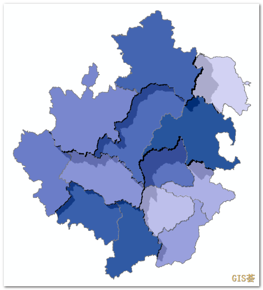
Drawing raster shadows based on input faceted vector elements, the tool creates a specific raster output by borrowing from the mountain shading method, and then simulates shadow casts of varying lengths depending on the value of the field attribute to express quantitative relationships between different element areas.
 |  |
|---|
The tool is borrowed from TerrainTool, with personal fixes and magic changes to the code and added instructions.
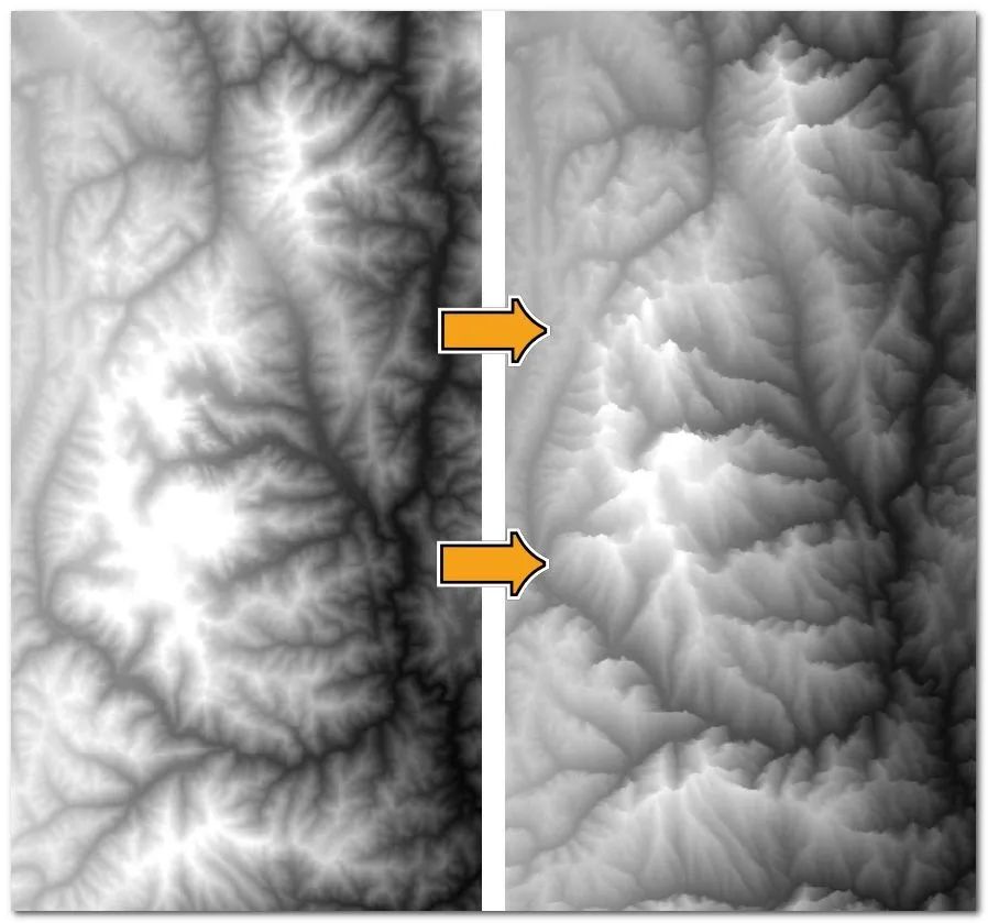
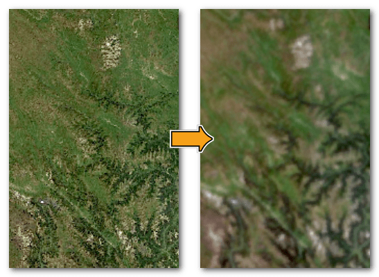
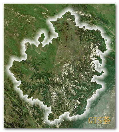
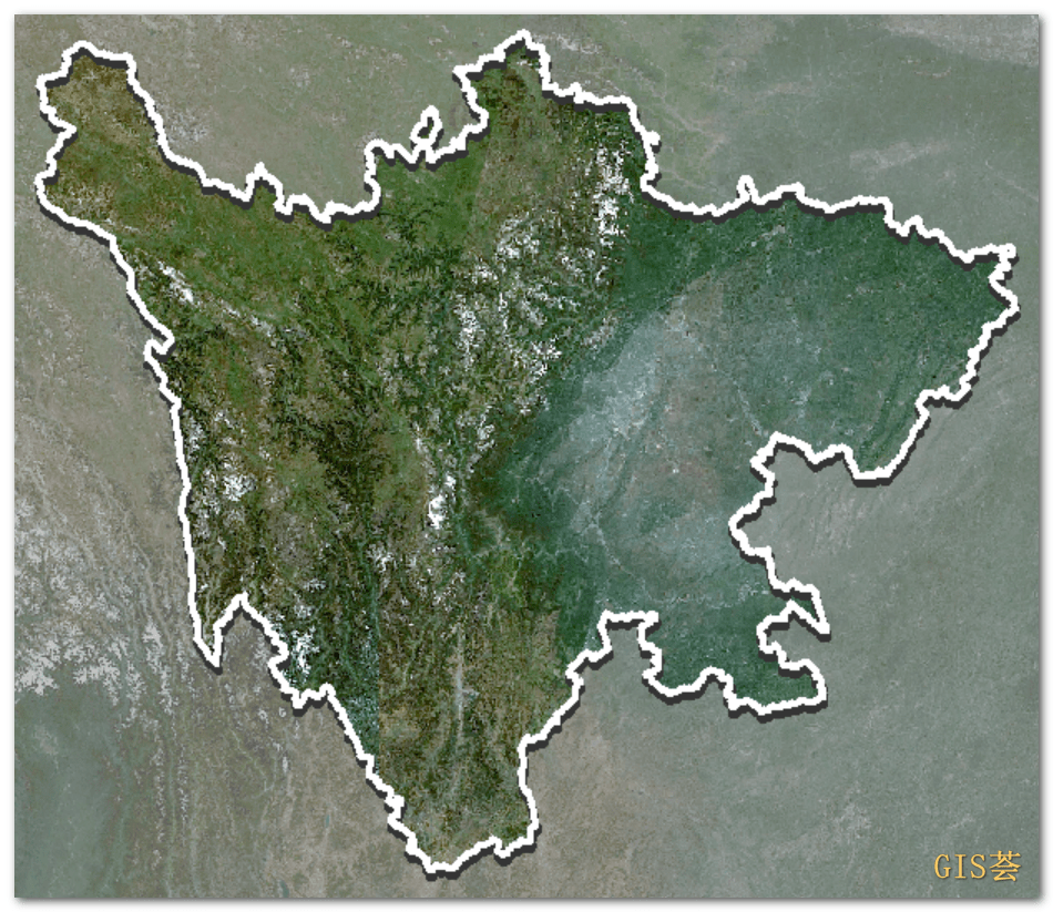
1.4 Background blurring
The input raster can be blurred. There are 1 to 5 levels, the higher the blurring level, then the higher the blurring of the output raster.
It can be used for the blurring of the background base map and the base map outside the study area. After the background blurring, the color tone of the resultant layer obtained may change, which can be adjusted by modifying the stretch type in the symbol system.
Due to the limitation of ArcPy function, it is known that ArcMap 10.1 and ArcMap10.2 do not support this tool, ArcMap 10.8.2 supports it, and the rest of the versions are not tested.
In conjunction with other outline styles, you can achieve the effect of focus highlighting in the study area.
2.Other tools available
| Note:For all the following tools, please make sure that the data is in the projected reference system before proceeding. |
I present each tool in turn, from top to bottom, according to the catalog structure of the toolbox.
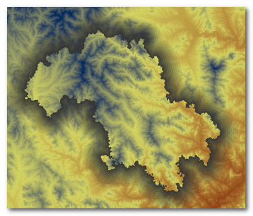
2.1 Bi-directional mountain shadows
Two solar orientation composite production of mountain shadows, both inherited ordinary mountain shadows (Hillshade) and multi-directional mountain shadows (Multidirectional Hillshade) advantages, but also to neutralize the shortcomings of the two, to avoid the loss of terrain details along the direction of the sun, to the light and the backlight of the terrain of the difference between light and darkness is particularly large; in addition to bidirectional composite production of the mountain shadows have a more In addition, mountain shadows made by two-way composite are more glossy and have better detail texture.
Bidirectional mountain shadows have less detail than multidirectional mountain shadows, so naturally the storage capacity of bidirectional mountain shadows is smaller (compared to multidirectional), and bidirectional mountain shadows are a compromise.
2.2 Multi-directional mountain shadows
Multi-directional mountain shadow rendering tool, ArcMap as well as ArcGIS Pro do not have a tool to directly produce multi-directional mountain shadows, while the built-in function method exists multi-directional mountain shadows.
So here is a step to the raster function implanted in the toolbox, directly produce multi-directional mountain shadows.
| Note:Multi-directional mountain shadows are darker in color and it is recommended to use standard deviation stretching in the symbol system and apply Gamma stretching to 1.3. |
Due to the limitation of ArcPy function, it is known that ArcMap 10.1 and ArcMap10.2 do not support this tool, ArcMap 10.8.2 supports it, and the rest of the versions have not been tested.
Below from left to right are the traditional effect, two-way mountain shadow effect, and multi-way mountain shadow effect (near Jianmen Pass, Guangyuan City):
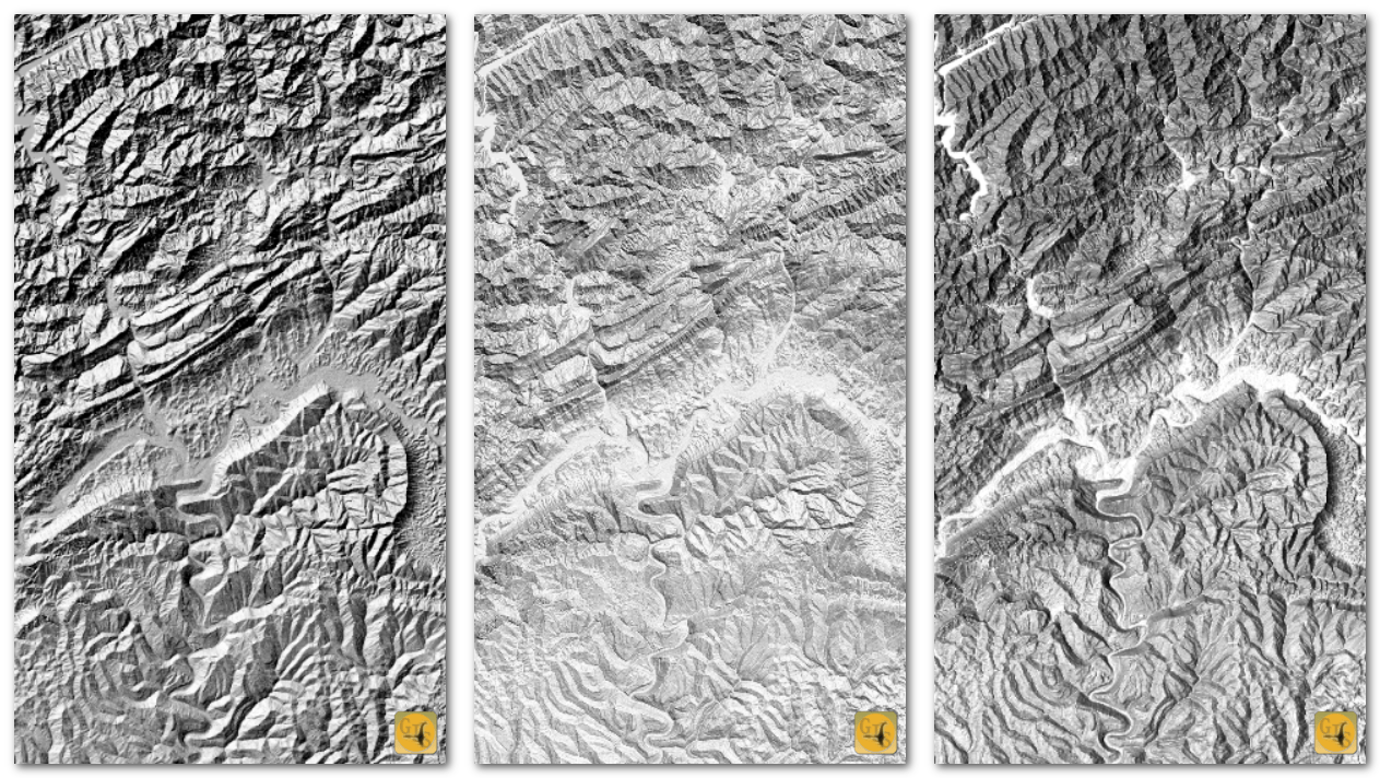
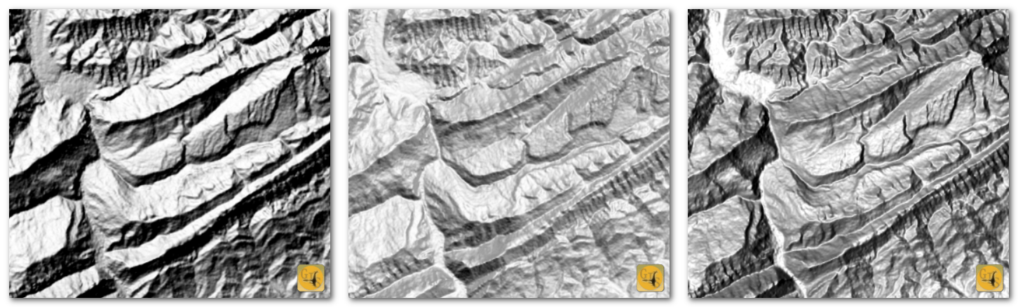
Conventional effect, bi-directional mountain shadow effect, multi-directional mountain shadow effect
2.3 Plane oblique axes diagram
New tools have been added and are described in detail in the first section.
2.4 light and dark contours
New tools have been added and are described in detail in the first section.
2.5 Better contours
Use the Focus Statistics tool to preprocess the raster data to produce better looking and smoother contours, as shown in the following figure, the left side is the contour generated by ArcGIS by default, and the right side is the contour produced by using the new tool, and you can clearly see the difference between the two.
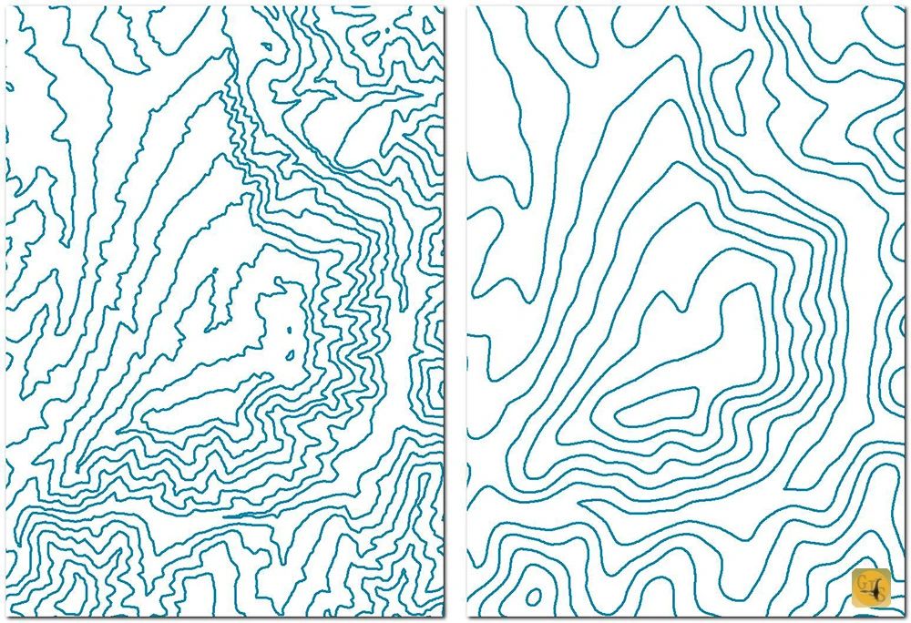
Left: organic matter contours generated by default; right: organic matter contours generated using the tool
2.6 Composite Gradient Offset
A variety of cartographic expression features from Cartographic Expressions, such as gradients and offsets, were used and finally combined with each other to create this effect.
Vector elements used for facets can highlight the extent of the study area or other areas that need to be focused on.
| Note:For mapping tools that use the graphical representation feature, the output file must be saved in the GDB database because of the limitations of the graphical representation itself. |
Left: initial; right: after using the tool
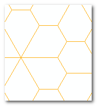
2.7 Tiled Pentagon 1
The Tile Pentagon tool creates pentagons with specific side lengths based on the extent of the input vector layer and tiles the entire extent.
In The Close Relationship Between GIS and Tiling and Tiling, the mathematical concepts related to tiled pentagons and their use in GIS are described in more detail, and how to use Python to call ArcPy to create tiled pentagons is also shared.
We also shared how to use Python to call ArcPy to make tiled pentagons, and made two different shapes of tiled pentagons, which are further encapsulated into a toolkit and integrated into the mapping style box.
| Note:When the data frame reference system does not match the layer reference system, running the tool may result in "Coordinates or measurements out of range". The simplest solution is to reopen an ArcMap, add data and run the tool. |
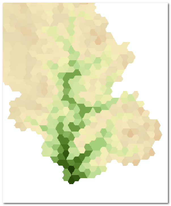
Statistical rasters for raster partitions made with the first kind of densely tiled pentagonal vector data
2.8Tiled Pentagon 2
Same as 2.7 Dense Lay Pentagon 1, the only difference being that the shape of the pentagon is different.
| Note:When the data frame reference system does not match the layer reference system, running the tool may result in "Coordinates or measurements out of range". The simplest solution is to reopen an ArcMap, add data and run the tool. |
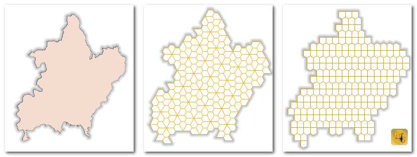
Left: input range; center: output of the first tiled pentagon; right: output of the second tiled pentagon
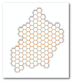
2.9 honeycomb hexagon
The Honeycomb Hexagon, also known as an isohexagon, is a tool that constructs a honeycomb hexagon based on the input to get a range of vector layers.
For users of lower versions of ArcGIS Desktop, higher versions come with their own hexagon creation tool: Data Management Tools->Sampling->Surface Subdivision Tool.
2.10 Building Shadows
A simplified version of the architectural shading created using the Cartographic Expressions feature, with an automatic default of 40% transparency.
| Note:For mapping tools that use the graphical representation feature, the output file must be saved in the GDB database because of the limitations of the graphical representation itself. |
2.11 relief effect
Embossing effect tool can be based on the input surface layer inward negative buffer to generate a raster layer, the size of the negative buffer distance needs to take into account the size of the input elements of the range, such as a county-level range of -1000 for the use of the buffer can be a better effect, remember to add the negative sign "-".
Embossed effect will be generated on the grid below the surface layer, the surface layer to set the transparency, you can get a "colored relief plate.
2.12 three-dimensional element
New tools have been added and are described in detail in the first section.
2.13 background blurring
New tools have been added and are described in detail in the first section.
2.14 light-emitting diode (LED) (Tw)
The outline glow effect, or feathering, created by combining the differential settings of transparency in a multi-ring buffer.
Create a multilayer buffer outside of the face element layer and then specify the transparency in turn to achieve the effect of glowing transparency. You can custom modify it to other colors.
| Note:The default effect is white, so you may not see the effect if there are no other background layers. |
The initial gradient interval distance is 10 meters, 90 meters in total, you can enter an integer value in the magnification field to make the luminous edge bigger.
The default magnification is 10, so the individual intervals are 100 meters, and the entire luminous outline is 900 meters. If you put in 2, it means the distance between the intervals is 20 meters, and the total luminous outline of the exterior is 180 meters.
If Beijing is such a large range of recommended 200, the specific size of the use of the situation.
Double click on the layer to open the symbol system, Elements->Single Symbol, which allows you to modify the color to other suitable colors.
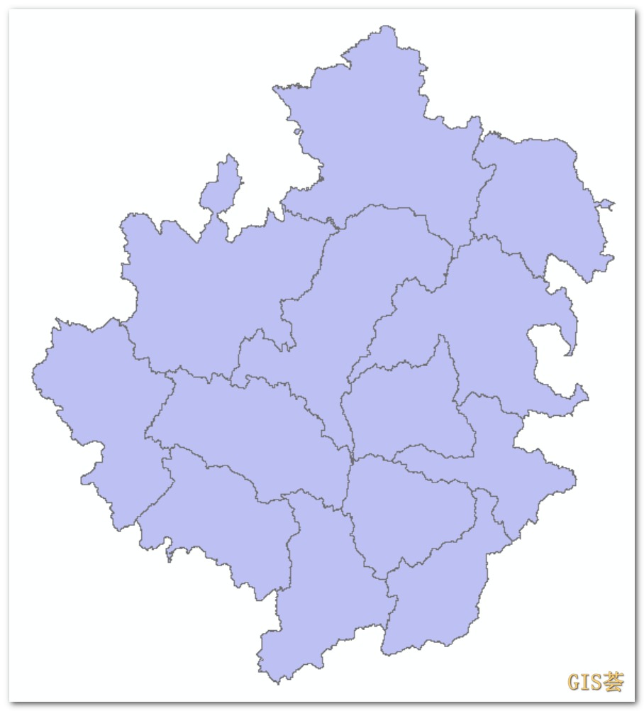
2.15 overall outline
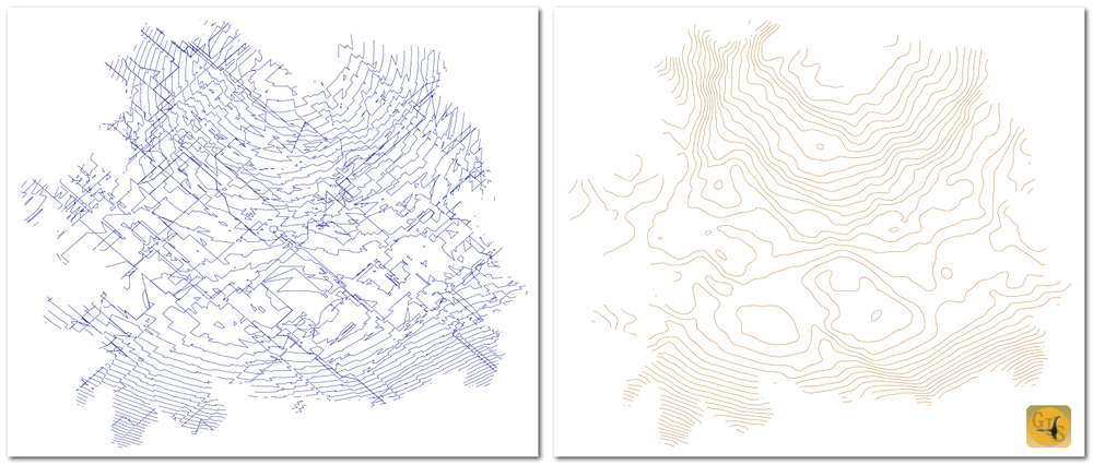
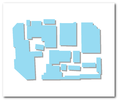
Using the Integral Contour Line tool you can merge one or more of the input element layers and completely eliminate the holes within.
It is quite common for elements to have holes in them, and when there are a lot of them, the elements look very fragmented. If the elements are mapped, e.g. contoured, then not only will there be generated contour lines on the outside, but the holes on the inside will be "crowded" with contour lines, which will make the whole map look dirty, especially if there are multiple layers.
This problem can be solved by using an overall outline.
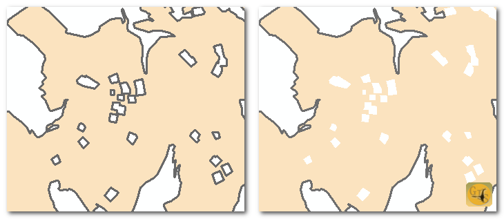
Left: before using the tool; Right: after using the tool
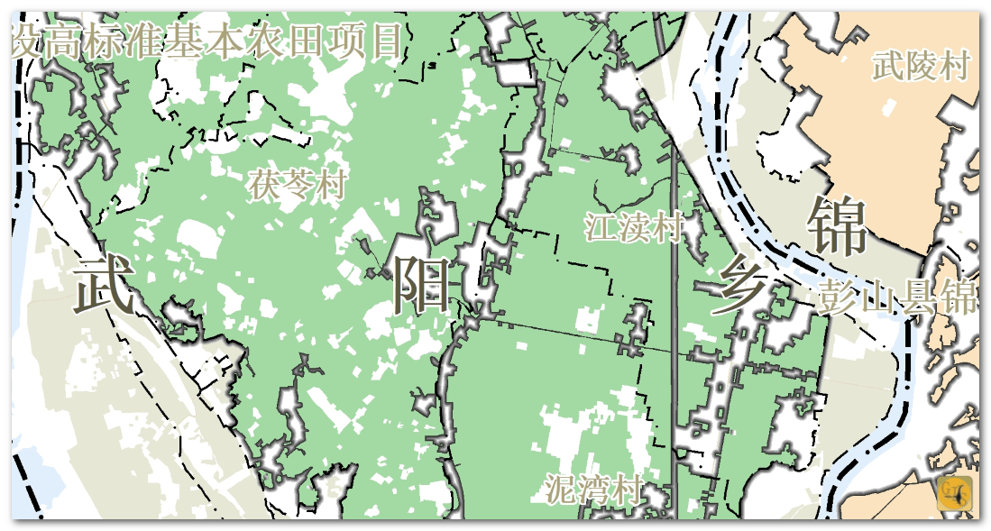
There are a large number of holes in the project location map of a certain area, the contour created by this tool can show the overall global contour without generating contours in each hole, ensuring a clear and concise map.
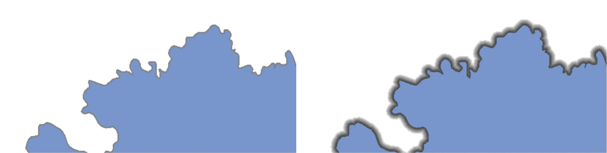
2.16 graduated outline
Achieve a uniform color gradient effect on the outside of the face layer through cartographic expression, with a black gradient by default, for both line and face vector elements.
| Note:For mapping tools that use the graphical representation feature, the output file must be saved in the GDB database because of the limitations of the graphical representation itself. |
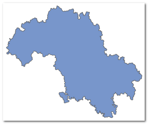
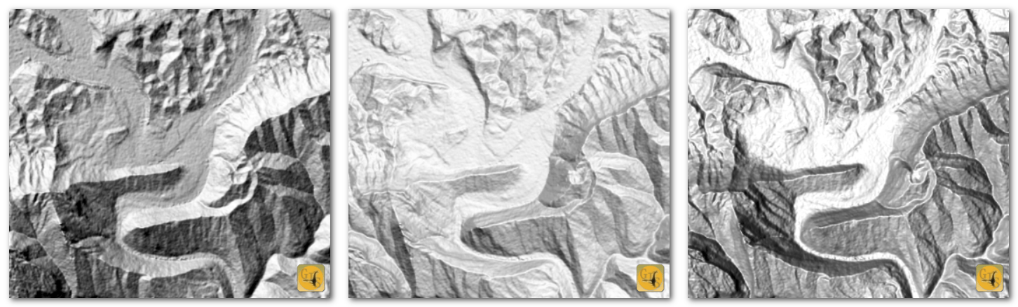
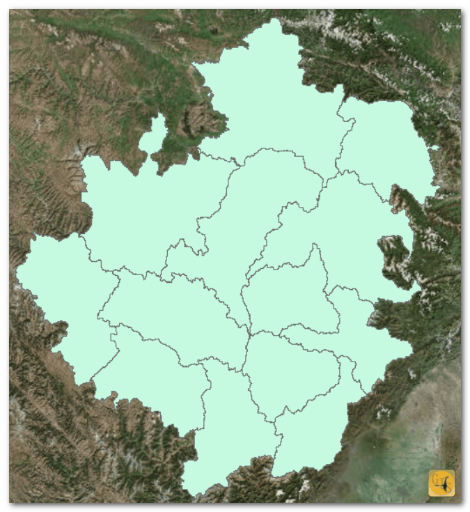
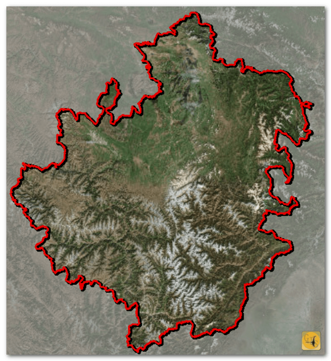
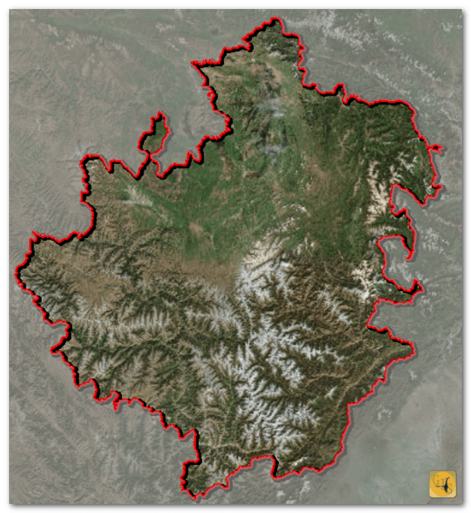
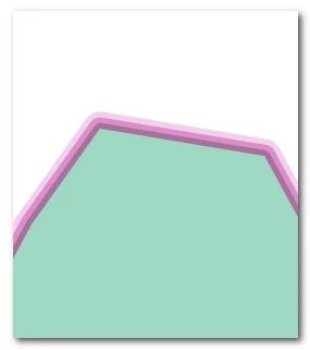
2.17 three-dimensional boundary (math.)
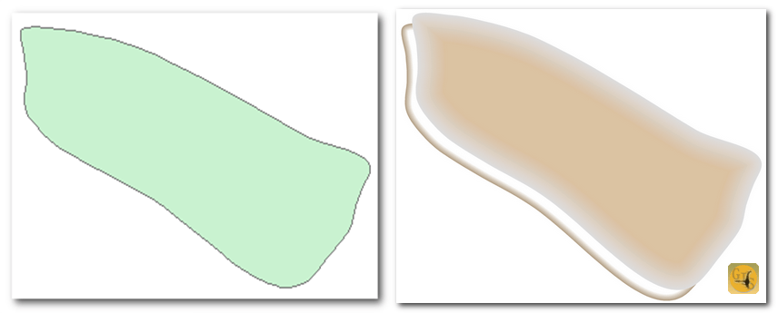
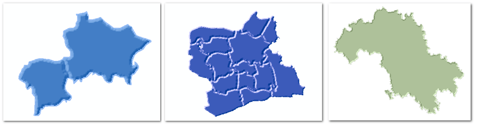
Obtain an offset boundary layer and a semi-transparent background layer (the area outside the project area) based on the input faceted vector data.
The default order is that the boundary layer is on top and the background layer is on the bottom; you can reverse the order and place the background layer on top, and you get the effect as in Figure 3, which gives a noticeable concave effect to the project area.
| Note:For mapping tools that use the graphical representation feature, the output file must be saved in the GDB database because of the limitations of the graphical representation itself. |
 |  |
|---|
The default layer order is border layer on top, background layer on the bottom (figure left); you can also adjust the order to put the background layer on top (figure right), which can make the project area have a noticeable concave effect.
In addition, you can also modify the color, after the tool is finished running, open the symbol system of the output layer, the cartographic expression item will appear, here you can modify the color of the border at will.
 |
|---|
2.18 buffer outline
Automatically merges all elements in the input face layer and outputs a complete three-level buffer contour. Default 30, 60, and 90 meter distance three-level contours.
The buffer distance of the buffer can be modified by adjusting the magnification.
The default buffer is 30 60 90 meters, when the magnification is entered as 10, a buffer of 300 600 900 meters can be obtained.
Buffer outline effect
3. How to use
How to use the GIS Aloe mapping toolbox, first of all, there are two compressed packages provided, one is StyleTool.zip and the other is Samples.zip;
Then there are two ways to add the toolbox to ArcMap.
3.1StyleTool.zip
After unpacking, you can see several folders: lyr, Representation, RasterFunction, etc., and the most important two toolboxes: GIS Aloe Mapping Toolbox.tbx and GIS Aloe Mapping Toolbox101.tbx.
Among the two toolboxes, the former corresponds to ArcMap version 10.8.2 and the latter corresponds to ArcMap version 10.1. Users with higher version can add the first toolbox, if you find that the tools are not complete after adding the toolbox, or you have a lower version of ArcMap, you can use GIS Aloe Mapping Toolbox 101.tbx.
3.2 Adding Methods
There are two ways to add GIS Aloe mapping toolbox to ArcMap.
Mode 1 Temporary addition: Open ArcMap software, in the toolbox window, right-click ArcToolbox to open the menu, and click the first item to add toolbox.
This is a temporary way, you need to add the toolbox again every time after restarting the software.
Mode 2 Permanent addition: Add to the toolbox system folder, the advantage is that the toolbox will be loaded automatically every time you open ArcMap.
Just unzip the contents of the GIS Aloe Mapping Toolbox.zip and copy them all to the ArcToolbox folder where the ArcGIS installation path is located.
Folder location (may vary depending on version and location of installation): C:Program Files (x86)ArcGISDesktop10.8ArcToolboxToolboxes
3.3 Samples.zip
Samples.zip contains sample data, such as vectors, raster data, and project files with .MXD extensions.
When you don't have existing data or the tool reports an error, you can open the project file with .MXD extension to see the effect, or use the data in the zip to run the toolbox to troubleshoot the error.
4. Applicable platforms
Toolbox in Win10 platform, all through the ArcMap 10.8.2 and ArcMap 10.1 test, all the tools can run normally, in addition to multi-directional mountain shadows and background blur does not support ArcMap 10.1.
At present, the toolbox does not support ArcGIS Pro, because the code platform has been upgraded from Python2 to Python3, and because ArcGIS Pro abandons the mapping expression function, extends the symbol system function, and has built-in many convenient mapping tools.
The mapping toolbox for ArcGIS Pro will streamline and add some new features that can only be realized by ArcGIS Pro, and it is still under preparation.
<
Comments are closed